
Defining Magnetic Properties
Refer to the Interface Reference Manual Materials section for more details about the implementation in TRAFOLO.
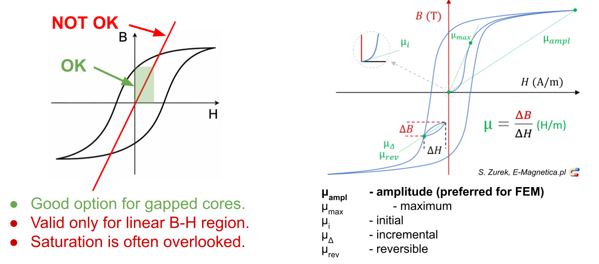
Constant Relative Permeability
Constant permeability is valid for the linear portion of the material’s B-H curve, far away from the saturation “knee.”
It is also suitable when most of the magnetic energy is stored in the air gap, making it sufficient for inductance calculations. When you introduce a physical air gap into a core, the total reluctance of the circuit becomes almost entirely dictated by the gap.
Complex Permeability
In real magnetic materials, when an alternating magnetic field (H) is applied, the resulting flux density (B) does not respond instantaneously. Due to internal loss mechanisms such as eddy currents, hysteresis, and microscopic relaxation effects, the B field lags behind H in time.
Complex permeability is an extension of constant relative permeability for AC (frequency-domain) analysis. While constant permeability assumes a fixed real value, complex permeability introduces a frequency-dependent, complex-valued parameter that captures both magnetic response and core losses. The B–H relationship is approximated as an ellipse, where the enclosed area represents energy loss per cycle.
Complex permeability models this behavior in the frequency domain by:
- Using a real part to represent energy storage (magnetic response)
- Using an imaginary part to represent energy dissipation (core losses)
This allows core losses to be inherently included in the material model, eliminating the need for separate loss formulations (e.g., Steinmetz models).
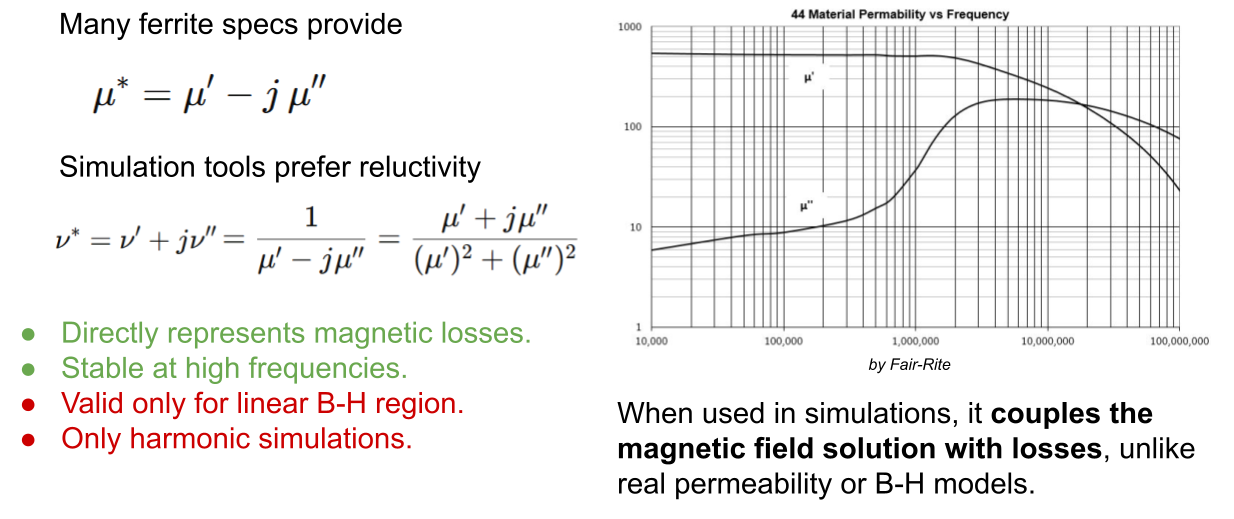

Complex permeability is based on a linear assumption. when operating near saturation, complex permeability may produce inaccurate results.
B-H curve
One of the primary benefits of the 3D Finite Element Method (FEM) is its ability to account for the material’s response to a magnetic field across the entire core volume. A hysteresis loop typically defines this response, which retains information about the material’s magnetic history and how the field has changed over time.
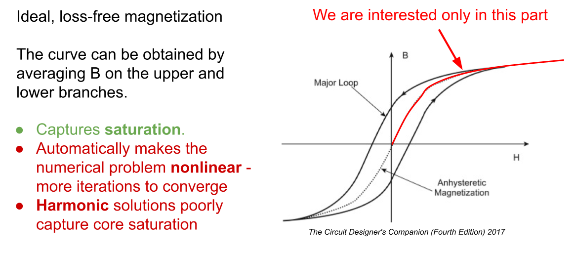
These B-H hysteresis curves are stored in separate files, with one column representing the magnetic field flux in [T] and the other representing the magnetic field strength in [A/m].
B-H hysteresis curves are stored in separate files with two columns, one representing magnetic field flux in [T] and another representing magnetic field strength in [A/m].
The use of B-H curve makes the numerical problem non-linear and requires more iterations to converge.
However, for 3D simulations, using hysteresis loops requires complex numerical techniques (such as the Jiles-Atherton model).
In ElmerFEM, as in most other FEM solvers, a simplified model is commonly used – a B-H curve that neglects coercivity and retentivity. This simplification focuses on the relationship between magnetic flux density (B) and magnetic field strength (H), but it does not store the material’s magnetic history, meaning hysteresis losses cannot be directly derived from the B-H curve in the simulation. Those losses are computed separately during a post-processing step.
Moreover, many material manufacturers either do not provide or are unaware of the B-H correlation for their materials. Additionally, measured data may contain outliers, leading to simulation convergence issues. For more details, check out our LinkedIn article discussing common B-H curve issues in FEM simulations: Fixing B-H Curve in FEM Simulations.
Algorithms to fix and extrapolate the B-H curve
TRAFOLO provides simple algorithms that improve B-H data. For example, to remove outlier points, it takes B-H data and derives Incremental permeability:
µi = dB / dH
Then, outlier points can be identified according to such conditions
- it cannot be smaller than 1
- sudden ups or downs
- incremental permeability in the saturation region should strive to 1
Additionally, you can smoothen the curve and extrapolate values into the saturation region. Users can choose to use the original or modified version of the B-H curve.
Use of B-H Curve for Harmonic Simulations
Usually, applying nonlinear B-H curves requires running time-domain (transient) simulations. Conversely, frequency-domain (time-harmonic) simulations are much faster but cannot account for non-sine material response for a sine excitation.
A common approach to deriving an equivalent B-H curve that preserves magnetic field energy compared to a transient solution is to use energy-averaging methods (e.g., “Simple Energy” and “Average Energy”) to generate cycle-averaged effective B-H curves, as illustrated in the COMSOL article Model Magnetic Materials in the Frequency Domain with an App.
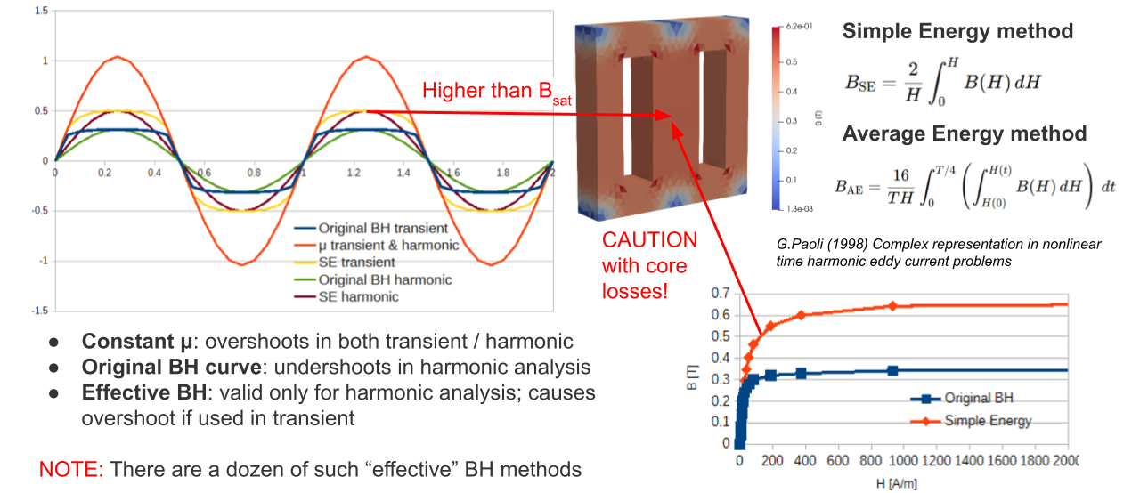
However, this method modifies the saturation region of the B-H curve, effectively extending it to higher values. As a result, special care is required when calculating core losses using Steinmetz models, as this may exceed the validity range of the coefficients and lead to overestimation of losses.
Lamination Stack Model
Due to their high permeability, laminated core materials exhibit small skin depth, which leads to significant eddy currents within the laminations. These eddy currents oppose the magnetic field, reducing the effective magnetic flux density and field strength in the core, particularly at higher frequencies.
To account for this behavior, a lamination stack model is used in FEM simulations. The model represents a frequency-dependent, anisotropic material in which the effective permeability decreases and magnetic flux penetration is reduced.
More details about the model’s implementation in ElmerFEM can be found in the article.
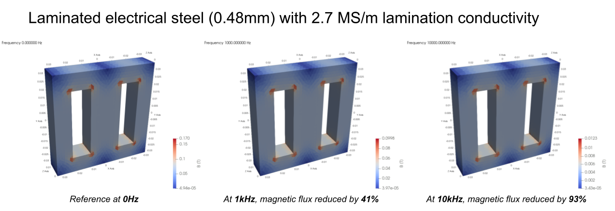
To illustrate the impact, a reference solution at low frequency (near DC) is shown on the left. At higher frequencies, the same core shows a substantial reduction in magnetic flux (1 kHz in the middle, 10 kHz on the right).
Permeability Gap
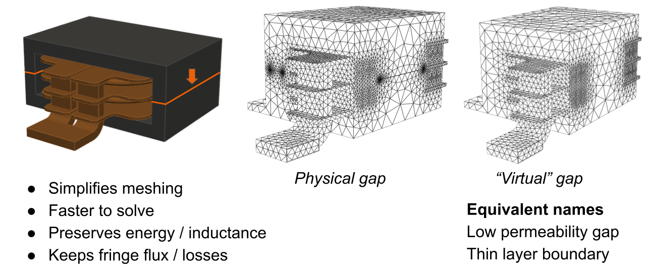
Very thin air gaps (or low-permeability regions) that are perpendicular to the magnetic flux lines can affect inductance and overall magnetic behavior. Accurately resolving these gaps with a mesh often requires extremely small elements, which increases computational cost.
To address this, a permeability gap model can be used. Instead of explicitly meshing the thin gap, the geometry is “sliced,” and a reluctance boundary condition is applied at that interface. This boundary condition represents the gap by defining its thickness and permeability.
Magnetization & Modeling Magnets
For magnet modeling in FEM, magnets are typically defined using remanent magnetization. This represents the magnetic state of the material after the external magnetic field has been removed. In other words, it is the operating point on the B-H curve at zero applied field, where the magnet still produces its own magnetic flux.
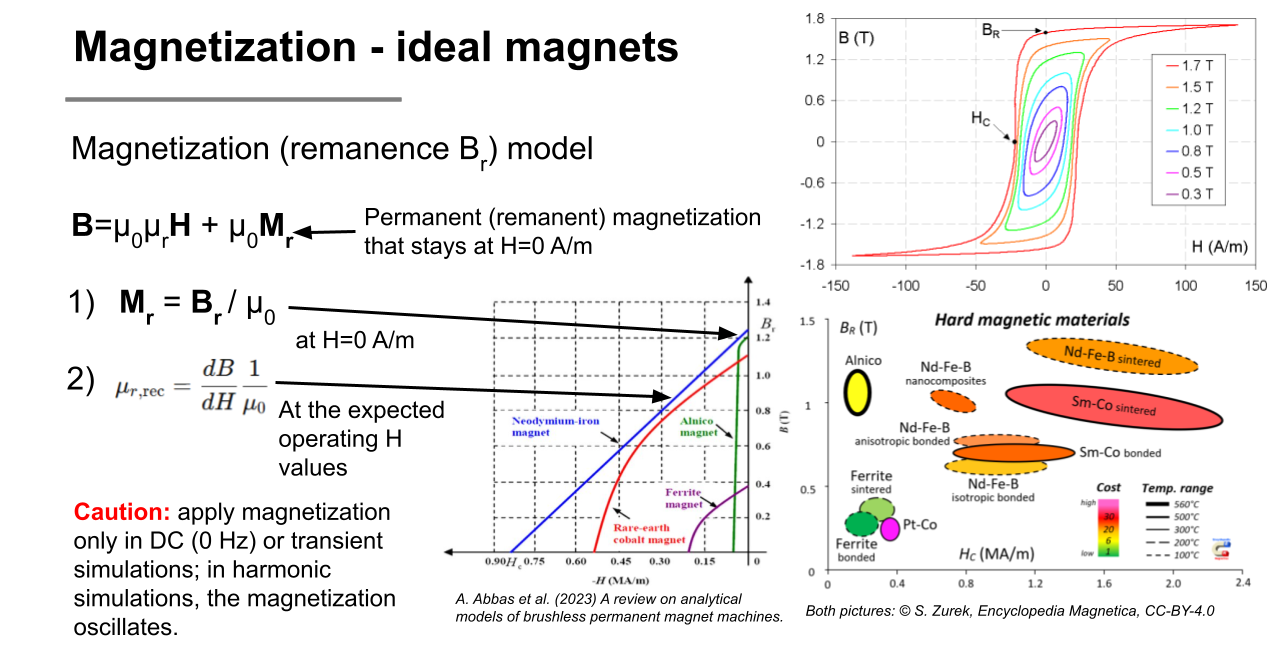
In practice, this remanent flux density (or equivalent magnetization) is specified as a material property. In addition, the magnet’s relative permeability must be defined. For most permanent magnets, this value is slightly above 1, meaning the BH curve slope is only marginally steeper than that of air. However, it does not inherently capture non-linear effects such as demagnetization under extreme conditions.
Special care is required for harmonic simulations – magnetization is treated as a complex quantity (with amplitude and phase), and the solver solves it as a time-varying property, effectively causing the magnetization to oscillate. While this can be useful for approximating rotating or oscillating magnetic fields, this is not physically correct for permanent magnets and can lead to inaccurate results.
Models Used for Core Loss Calculation
Complex Permeability
Core losses are calculated during the electromagnetic simulation. This approach is particularly suitable for high-frequency applications (e.g., ferrites) under linear or small-signal conditions.
The solver uses the imaginary part of the permeability to determine the loss generated in the magnetic material at a given frequency. This loss typically includes both hysteresis and eddy losses.
Unlike Steinmetz-based approaches, which estimate losses after the simulation, complex permeability:
- inherently accounts for losses and magnetic field attenuation (shielding)
- provides direct feedback to the electrical circuit, reflected in quantities such as frequency-dependent (AC) resistance via complex voltage and current
Methods based on the Steinmetz equation
For harmonic simulations, the same Steinmetz + Eddy equation is applied during the processing step to calculate losses at all frequencies independently, and then the results are summed (superposition principle). This assumes that losses at different frequencies are independent.

Due to the nonlinear nature of the B-H curve and the dependence of core losses on magnetic flux and frequency, this assumption is an approximation that can sometimes lead to significant errors. We recommend validating core losses with transient simulations, especially when core losses are critical
