
In the TRAFOLO Setup window, you can configure several key settings, such as domain type and numerical models, which will impact the subsequent workflow, computational time, and accuracy of your simulation.

General
Domain Type
Symmetric – Used when the model’s geometry can be divided into two symmetric parts along the XY plane (same as Z=0). The use of symmetry not only reduces the problem size but also greatly improves the convergence rate, so it should be applied whenever possible. Parameters like voltage, resistance, losses, and inductance are scaled to represent the values for the full geometry.
After assembly (cutting by symmetry plane), all winding geometries must have at least two terminals on the symmetry plane, and the magnetic flux should be parallel to the symmetry plane.
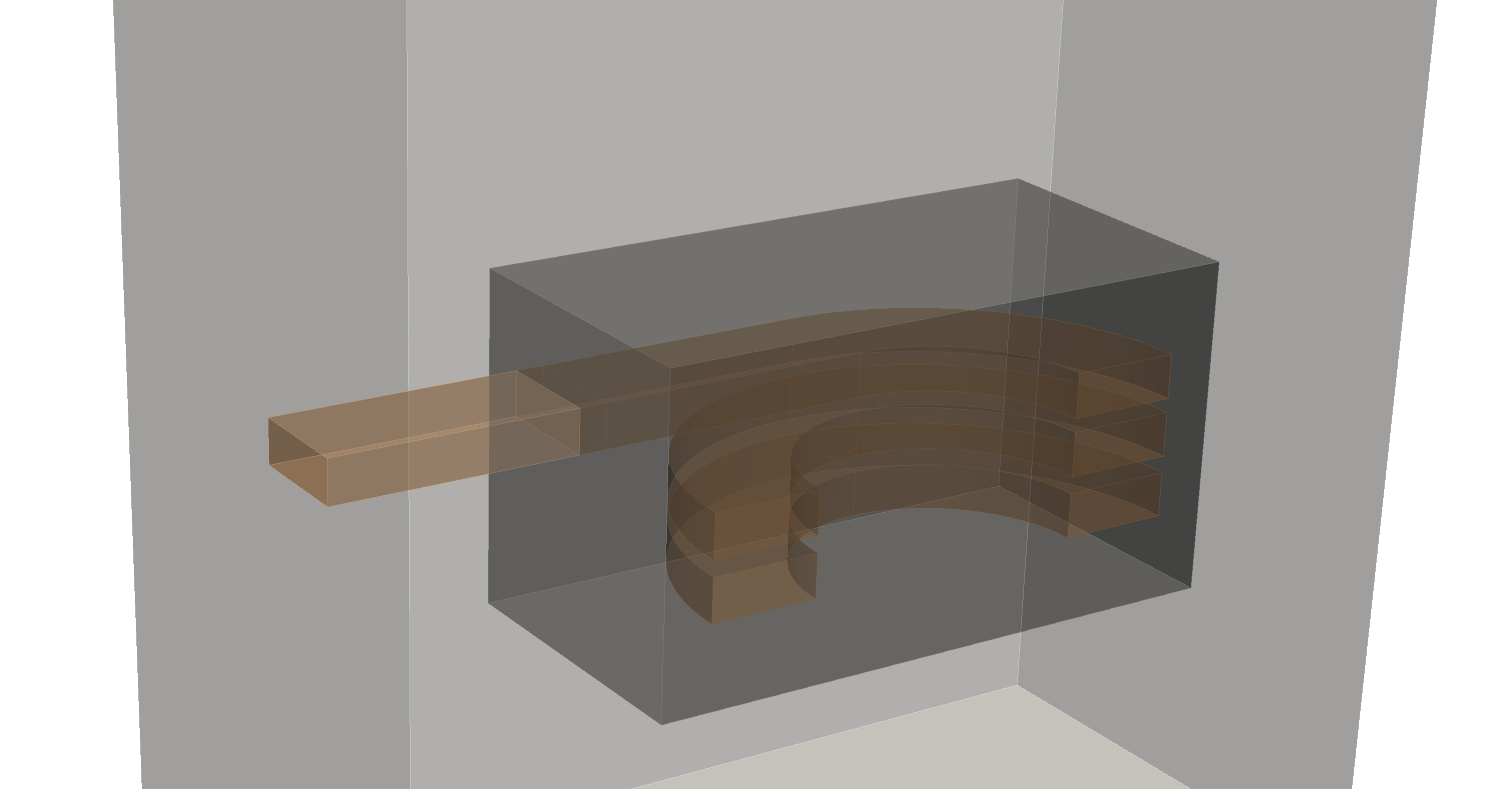
Full – Use when symmetry is not possible. Simulation times may increase, and convergence may be slower, especially for windings with solid (massive) conductors and many turns. For stranded (litz) wires, a closed coil can be defined by enabling the Closed Coil option in the coil settings. For other conductor types (solid/massive and foil), closed coils are not currently supported. In these cases, the winding must be cut, with at least two terminals extending to the domain boundary.

Simulation type
TRAFOLO supports both steady-state and transient analyses for electromagnetics and heat transfer. When both types of analyses are enabled, automatic coupling is established between the two domains, ensuring seamless integration. This coupling is performed in a weak coupling manner, where the electromagnetic and heat transfer analyses are solved sequentially. Losses from the electromagnetic simulation are transferred to the heat transfer simulation, and the resulting temperature distribution is sent back to the electromagnetic solver to update temperature-dependent properties. All coupling directions are illustrated in the scheme below.

Electromagnetics
Transient – Used for non-sinusoidal waveforms or non-linear scenarios where sinusoidal excitations produce non-sinusoidal responses, such as in saturated cores where the B-H hysteresis curve exhibits strong non-linearity.
IMPORTANT:
- Transient simulations are affected by inrush currents and voltages. In all simulations, the initial magnetic flux is set to 0T. To minimize inrush effects, ensure that the magnetizing current at time 0 is minimal, or when using the voltage as excitation, set it to a value corresponding to the phase where the current is 0 (typically at the maximum voltage value). More info in the article.
- The lowest frequency and number of periods determine the simulated time, while the timestep size depends on the highest frequency. For example, in case of 50Hz fundamental frequency and 1000Hz as a harmonic and a minimum of 20 points per period, the total number of time steps required will be 1000/50*20=400. When there is a significant difference between the lowest and highest frequencies, it is recommended that the transient simulation be harmonized. It can be done in the Waveform tab.
Harmonic – Used for sinusoidal waveforms, magnetostatic simulations (0 Hz), and cases involving multiple independent harmonics. Total losses are computed as the sum of the losses for individual harmonics, with RAC calculated separately for each frequency. Further, Transient simulations can be converted to Harmonic simulations using the DFT functionality under the Waveforms tab.

Harmonic simulations may produce inaccurate core loss results, as core losses are inherently non-linear, making harmonic superposition invalid. In addition, DC bias effects in the core are not captured.
Inductance – Conducts a sweep analysis based on harmonic simulations to calculate inductance, reactance, Q-factor, losses, and other related parameters across different current, voltage levels, or frequencies.
Phases – Specifies the number of phases for current or voltage sources. For three-phase cases, a 120-degree angle is set between sources.
Capacitance – A separate electrostatic simulation determines the capacitance matrix between coil groups. From it, TRAFOLO calculates the interwinding capacitance between the primary and secondary windings. Intrawinding (self) capacitance is calculated using a different setup: enable Without Circuits and solve for the full domain, including the coil.
Capacitance depends on the permittivity of the dielectric materials surrounding the windings. To account for this, use the bobbin geometry to fill the space between conductors and assign it an effective permittivity. Perform mesh refinement between the turns or windings used for capacitance calculation. If additional local refinement is needed, apply it to the bobbin geometry.
Without Circuits – The electrical potential (voltage) is applied directly to the winding terminals, bypassing the need for circuit connections. This option also allows calculation of the self-capacitance of a winding. When solving imported solid multi-turn windings at high frequencies, where the skin depth is significantly smaller than the wire cross-section, the numerical solver may struggle to converge. This issue can be mitigated and convergence improved by skipping circuits.
This option is only available for full domains and inductance calculations. Enabling this option limits excitation to voltage only, as current inputs are not supported.
Heat transfer
The heat transfer model in TRAFOLO primarily focuses on heat conduction in the component while incorporating heat transfer boundary conditions and the Stefan–Boltzmann law for radiation on its external surfacres. Note that this approach allows for very fast thermal simulations, but incorporating convective heat transfer necessitates determining heat transfer boundary coefficients using empirical models or prior experience.
Transient – This type of simulation is used for time-dependent heat transfer simulations. It requires solving many time steps, making it longer than a steady-state thermal simulation. It is useful for comparing measured data with simulation results when reaching steady-state temperature takes too long or when the thermal inertia of the component must be considered.
Steady-state – Used for solving temperature in a stationary state. It represents operations where the temperature distribution has reached equilibrium and losses are balanced with heat removal from the component.
Temperature iterations – This option is only available for Steady-State heat transfer. By setting this value greater than one, the software transfers the solved temperature distribution from the heat transfer simulation back to the electromagnetic solver, allowing it to account for the temperature dependency of material properties, such as electrical conductivity. This iterative process ensures that temperature effects are incorporated into the electromagnetic calculations for greater accuracy.