
Additionally, TRAFOLO does not use computational fluid dynamics (CFD) solvers to account for convective flows, which are typically part of complex and time-consuming Conjugate Heat Transfer (CHT) simulations. Instead, TRAFOLO employs a simplified approach using heat conduction within solids and heat transfer boundary conditions on external surfaces, allowing for faster simulations that still provide sufficient accuracy for many cases.
In the Heat tab, users can assign thermal boundary conditions to external surfaces and set heat sources within the component bodies.

The decision between transient and steady-state heat transfer simulation should be based on the time and spatial scales of the component. Smaller components typically reach thermal equilibrium more quickly due to lower thermal inertia and shorter characteristic lengths. For such cases, steady-state solvers may suffice.
However, larger components may take hours for heat to saturate because of their greater thermal mass and lengths for what to transfer. In these cases, transient simulations are more suitable, as they allow for real-time observation and comparison of temperature changes against measurements, accounting for both conduction and thermal mass effects.
Without Heat Transfer
Steady-State Temperature – Sets the temperature for temperature-dependent material properties (e.g. conductivity). Run a preliminary simulation to estimate the value or make your best guess.
Transient Heat Transfer
Initial Temperature – At the start of the simulation (t=0s), all components will begin with this initial temperature. As the transient heat simulation progresses, the temperature will adjust accordingly, influenced by the applied boundary conditions and any defined heat sources.
Timesteps – These are the time points at which the solver computes the temperature. Smaller time step sizes are typically used at the start of the simulation to capture rapid temperature changes, with step sizes increasing as the system approaches thermal stability. The Generator can set evenly-spaced timesteps, but it’s better to manually adjust for shorter steps during rapid changes and longer ones as the temperature stabilizes.
Steady-state Heat Transfer
Predicted Steady-State Temperature – This provides an initial estimate for temperature-dependent material properties in electromagnetic simulations. Considering that temperature-dependent properties lag behind the temperature solution, you can run a preliminary simulation to estimate the value or set the Temperature Iterations in the Setup tab to greater than one. This allows the temperature results to be passed back to the electromagnetic solver for further correction.
Boundary Conditions
When Heat Transfer is activated in the Setup section, all external faces of the component are displayed here. You can select a body or face from the list, and click on the preview to adjust the boundary condition type to the one that best suits your simulation needs.
Type
- Fixed Temperature forces a boundary condition to have a constant temperature.
- Heat Flux specifies how much heat energy enters or leaves a system through the boundary. It is defined as the rate of heat energy transfer per unit area.
- Insulation – zero heat flux (adiabatic condition).
- Convection type imitates a convective heat removal from external surfaces. It is modeled using external temperature (of air, liquid, etc.) and heat transfer coefficient, indicating heat removal’s efficiency. Heat transfer coefficients depend on the type of heat transfer mechanism, material properties, and the nature of fluid flow (if applicable).
Heat transfer coefficient – Naturally cooled applications by air are typically set to 5-10 W/m2/K, but it increases with the forced flow or changing air to liquid. These coefficients can be empirically estimated.
- Air at free convection: 2.5–25 W/(m2K)
- Air at forced convection: 10–500 W/(m2K)
- Liquids at forced convection: 100–15000 W/(m2K) Use QuickField, an online calculator, to estimate values:

Idealized Radiation Model – The Gray Body Radiation model defines emitted thermal radiation at a rate proportional to their emissivity, which is always less than 1. The net Radiation Loss Rate is calculated as follows
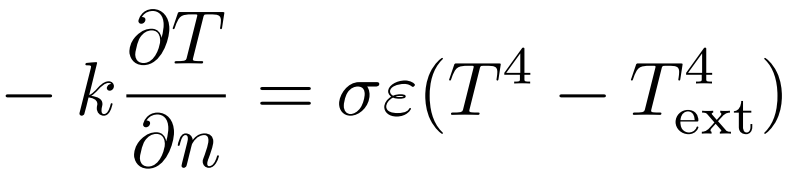
where σ is the Stefan-Boltzmann constant and ε the surface emissivity.
Emissivity – The coefficient defines the effectiveness of a material’s ability to emit/absorb thermal radiation, and it depends on material and surface properties. Some common materials and their emissivity coefficients can be found here.
Heat Sources
This option is available when the electromagnetic solver is disabled, allowing the user to apply a homogeneous heat source or sink to a specific part of the component. To do this, select the desired part in the geometry preview window and specify the power in watts (positive for heat sources, negative for heat sinks).

The Heat Source setup is only accessible when electromagnetics is not being solved in the Setup tab. The user should either input their own losses or run the electromagnetic simulation to pre-compute the losses, and then proceed to use the heat transfer solver independently.

Total Group Power – This setting applies a uniform distribution of heat sources (or sinks, if negative) across the selected group or its individual components. The power is distributed proportionally based on the volume of each part.