
The Material Library in TRAFOLO provides data for both electromagnetic and thermal analysis. It includes a wide range of materials sourced from databases and online resources and is regularly updated.

Global Materials – These are shared across all simulation cases and users (if multiple users share the same TRAFOLO installation). Materials shown in bold are the default ones provided with the software and cannot be modified. User-added materials, not in bold, can be edited. By default, global materials are stored in: C:\Users\%username%\AppData\Roaming\Trafolo\materials.
Local Materials – Add all the materials required for a specific simulation to Local Materials. These will appear in the Default Material section and the Assembly tab. They are only available for the specific simulation case and are stored in the case folder.
Default Materials – You can optionally assign default materials here, which will automatically be applied to corresponding components in the Assembly tab. The default material can be overridden later within the Assembly tab if needed.
Copy – Duplicates materials between the Global and Local databases. To copy, select the material and click the Copy button.
- Right arrow – copies material from the Global to the Local database.
- Left arrow – moves material from the Local to the Global database.
Editing Material Properties
Material type – The software uses different numerical methods and parameters depending on the material type to calculate losses and responses to electromagnetic fields. For instance, core materials require core loss data, whereas general materials might have a temperature coefficient for electrical conductivity.
General Properties

Core Material Type – This field is only visible when selecting a Core material type. Different core materials, such as laminated electrical steel and ferrites, require specific material properties. They utilize distinct numerical models to calculate losses and their response to magnetic fields.
Laminate Stack Conductivity – This field is available only for Laminated Core materials and is used to adjust the permeability of laminated materials at high frequencies. It requires setting the electrical conductivity for the lamination material. The temperature dependency of conductivity is not considered.
Electric Conductivity – used to calculate eddy currents and losses in the core.

When simulating non-laminated cores with non-zero electrical conductivity, the 3D solver will explicitly calculate macroscopic Joule (resistive) losses caused by internal eddy currents. However, standard empirical core loss formulas (like the Steinmetz equation) are derived from manufacturer measurements that already include material-level eddy current losses. To prevent double-counting these losses, engineers must be extremely careful; if you rely on a Steinmetz model for total core loss, you must either set the bulk core conductivity to zero, or use modified Steinmetz coefficients that strictly isolate hysteresis losses.
Laminate Thickness – This field is visible exclusively for Laminated Core materials and requires lamination thickness in mm as an input. It works in conjunction with the Laminate Stack Conductivity.
Temperature coefficient – α is temperature-dependent electrical conductivity approximated as linear dependence:
σ = σ0
where σ0 is electrical conductivity at 20 °C, T is solution temperature, and T0 is the constant temperature at 20 °C.
TRAFOLO uses weak coupling between electromagnetic and thermal simulations. The first EM solution is based on the Initial Temperature from the Heat tab. With Temperature Iterations > 1 provided under the Setup tab, later EM iterations incorporate temperatures calculated by the thermal analysis.
Defining Magnetic Properties
More details on the models used are in the User Manual, Core Properties and Losses section.
Three models are available for describing magnetic material properties:
- Relative Permeability (constant)
- Complex Permeability (frequency-dependent)
- B–H curve
For more detailed information about the use of different models, refer to the Users Manual’s Core Properties and Loss section.
B-H curve
You can import B-H and H-B curves. TRAFOLO will identify the type based on amplitudes. Once the data is imported, you can modify the B-H table values.
Ensure your data file contains two columns separated by a delimiter (e.g., comma, space, tab, or semicolon). Use SI units – Magnetic flux density (B) should be in teslas [T], and magnetic field strength (H) should be in [A/m].
B-H Curve Optimization – Once the curve is imported, TRAFOLO will remove outlier points (line name “Fixed”) and extrapolate to saturation (line name “Fixed + Extrapolated”), assuming that the differential relative permeability at high magnetic strength tends to 1.
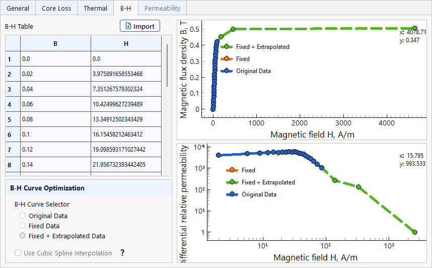
Use Cubic Spline Interpolation – By default, linear interpolation is used to fill in the gaps between sparse data points in the B-H curve. This option enables higher-order interpolation that smooths out the curve, making it easier for nonlinear solvers to converge faster in some cases.
TRAFOLO supports most text file formats (CSV, txt, etc.). If you get an error during import, save the file in a different format or try a different delimiter.

Complex Permeability
Values can be copied from a spreadsheet or tab-separated text. Fill in all three columns – Frequency, Real, and Imaginary. Ensure there are no empty cells.
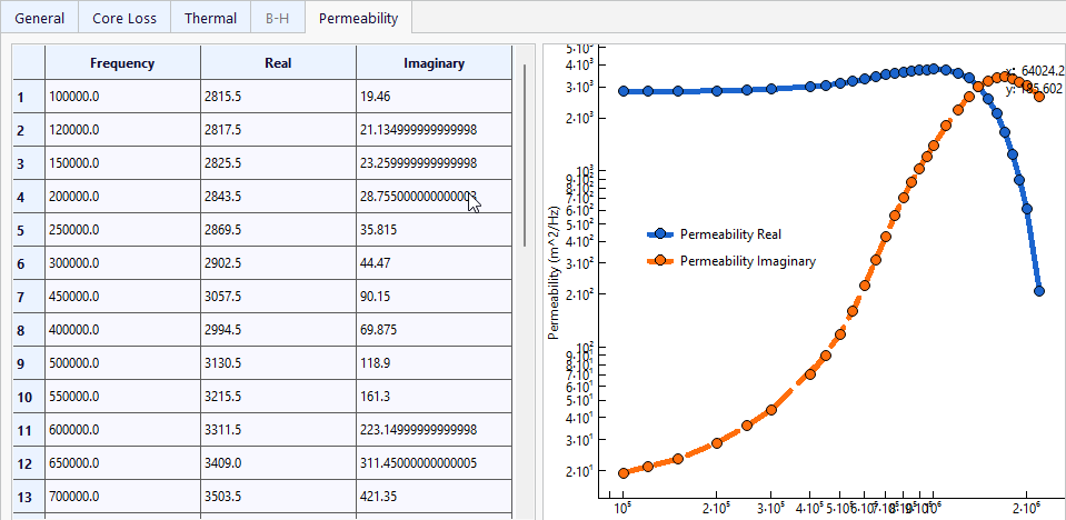
Complex permeability is used only in Harmonic simulations (including Inductance simulation type). Since core losses are included in the imaginary part of the complex permeability, Steinmetz-based loss models are disabled.
Core Loss
Core losses are defined using Steinmetz-type equations and calculated during the postprocessing stage using magnetic flux values and frequencies (for harmonic cases) or time derivatives of the magnetic flux (for transient cases).

Core loss data is usually provided as P(f, B) tables, with f in Hz and B in teslas.

Prepare your core loss data table in most text file formats (CSV, txt, etc.), with columns and rows defined by frequency in Hz and magnetic flux density in teslas (T). Based on amplitudes, TRAFOLO can identify automatically which column or row corresponds to the frequency and magnetic flux values.
Units may include W/kg, mW/cm³, or W/m³. TRAFOLO fits this data on the 4-parameter Steinmetz + Eddy Equation:

where four coefficients that are obtained for every material are
- Kh – the coefficient is related to the hysteresis part of the total core loss.
- m – exponent for frequency, typically around 1.
- n – exponent for magnetic flux density, typically around 2.
- Ke – the coefficient is related to the eddy current part of the total core loss.
Frequency Range – With this range, you can restrict the frequency used for fitting to improve accuracy. Curve-fitting non-linear core loss data over a wide range of frequencies and B-field amplitudes using a standard 4-coefficient model often yields poor mathematical fits. This causes the simulation to drastically over-predict or under-predict core losses at certain operating points.

Thermal Coefficients – Scales losses based on temperature (°C). Ensure temperature coefficients use the same reference temperature.
More details on the models used are in the User Manual, Core Properties and Models section.
Thermal Heat Transfer
Density – This parameter is used to convert core losses between W/m³ and W/kg and plays a role in modeling transient heat transfer, where it contributes to thermal mass (related to heat absorption). For steady-state thermal simulations, this parameter does not affect the results.
Heat Conductivity – One of the most critical parameters in thermal simulations, it determines how heat is transferred within the component. Since thermal conductivity can vary by more than three orders of magnitude between different materials (e.g., 400 for copper and about 0.2 for epoxy resin), it is particularly essential to account for thermal conductivity in dielectric materials. Additionally, thermal conductivity can be anisotropic, meaning it varies by direction. This value is a scalar for homogeneous materials, while for non-homogeneous materials (e.g., laminated cores), it can be expressed as a vector (kx, ky, kz).
Heat Capacity – Similar to density, this parameter contributes to thermal mass and is crucial in transient thermal simulations.