
The Waveform tab is used to define the electrical excitation amplitude applied to your magnetic component. TRAFOLO adapts the interface depending on whether Transient or Harmonic simulation type is selected in the Setup tab, allowing you to define waveforms parametrically, load external measurements, or set up a harmonic spectrum.

The interface also allows converting transient waveforms into the frequency domain by decomposing them into harmonics using the Discrete Fourier Transform (DFT).
Harmonic Excitation Configuration
Used for excitations that can be represented by a few independent harmonics, particularly when the fundamental frequency and higher-order harmonics differ by orders of magnitude, making transient simulation impractical due to the large number of required time steps.
When using the B-H curve, TRAFOLO assumes the fundamental frequency has the highest amplitude, and the corresponding amplitude permeability is fixed for subsequent harmonic calculations.
Magnetic fields, current amplitudes, and losses are then computed using superposition by summing the contributions of individual harmonics. If accurate core loss estimation is critical, we recommend running a separate transient simulation to quantify the difference from the harmonic approach. A further option is to export time-dependent magnetic flux at several characteristic points to evaluate it with an iGSE model and compare it with the locally averaged losses for reference.
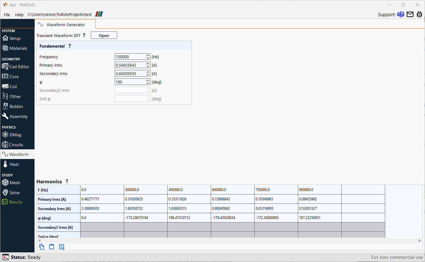
Transient Waveform DFT – Opens a separate window to convert imported transient waveforms (amplitudes and phases) into multiple harmonics using the Discrete Fourier transform.
Fundamental – It is assumed that the fundamental frequency has the highest amplitude. The key difference compared to harmonics is that the permeability calculated at this frequency is then applied to all other harmonics.
In TRAFOLO, all RMS values are labeled with the suffix “rms.” Values without it represent amplitudes.
φ / 2nd φ – Relative phase shift between primary and secondary windings. As harmonics are treated as independent, all primary harmonics are assumed to have zero phase by default (source is purely real).
IMPORTANT:
- This is not an absolute phase but rather the difference between secondary sources and primary. Although the relative difference is sufficient for calculating Rac/Rdc, losses, and other frequency-dependent parameters, you cannot reconstruct the initial waveform from these harmonics.
- Phase shift does not consider terminal selection. Swapping the positive and negative terminals effectively will change the phase shift 180 degrees.
Harmonics – A table defining harmonic frequencies, RMS amplitudes, and phase angles. Each harmonic is independent, with a separate EM simulation per frequency.
IMPORTANT: Avoid adding harmonics that would produce negligible losses to reduce simulation time.
Values in most tables can be copied and pasted directly from a spreadsheet program (e.g., Excel or Google Sheets).
Transient simulations
Transient simulations are used for non-sinusoidal waveforms or non-linear cases where sinusoidal excitations result in non-sinusoidal responses, such as in saturated cores with a strongly non-linear B-H hysteresis curve.
When harmonics differ by orders of magnitude, low frequencies set the simulation length while high frequencies set the timestep. This can lead to impractically large simulations (e.g., 50 Hz + 10 kHz requires long duration and fine resolution). In such cases, harmonic simulation is recommended.
The selector at the top chooses the waveform source:
- Generate Parametrically – transient waveforms created using simple shapes.
- Load from File – waveforms imported as time series from SPICE or alternative.
We begin with the common settings and then cover the differences.
Frequency – typically represents the lowest resolved frequency (usually the fundamental), as it defines the period length.
Periods – The total number of periods to simulate. The period length is determined by the frequency.
Skip Periods From Averaged Losses – The number of periods the solver ignores before calculating averaged losses. Initial timesteps in transient simulations often contain higher errors due to phase mismatches between voltage, current, and magnetic flux, as well as inrush currents.
Generated Waveforms
When Generate Parametrically is selected, the user can create waveforms using simple shapes such as sine, square, or triangular. Waveforms for primary and secondary are defined separately.
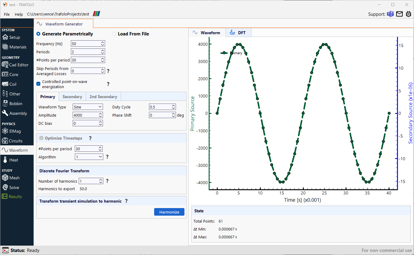
Points per period – defines the resolution of the generated waveform.
In 3-phase cases, only one waveform is shown. The other two are automatically generated with a 120° phase shift.
Controlled point-on-wave energization – Setting is available only for 3-phase models. It enables controlled energization of each phase to minimize inrush current. Steady-state (harmonic) conditions are typically reached within one period, after which parameters and losses can be evaluated. More details in the article about modeling 3-phase components.
Imported Waveforms
When Load From File is selected, the user can import waveforms from SPICE or equivalent circuit simulators. TRAFOLO supports most text formats (CSV, TXT, etc.) as well as Excel files.
TRAFOLO assumes the first row contains column names. After importing the waveform, select the time series and sources based on these column names.
If import fails, try a different file format or delimiter. Make sure all rows contain the same number of columns, and check for special characters or conflicts between decimal and column separators.
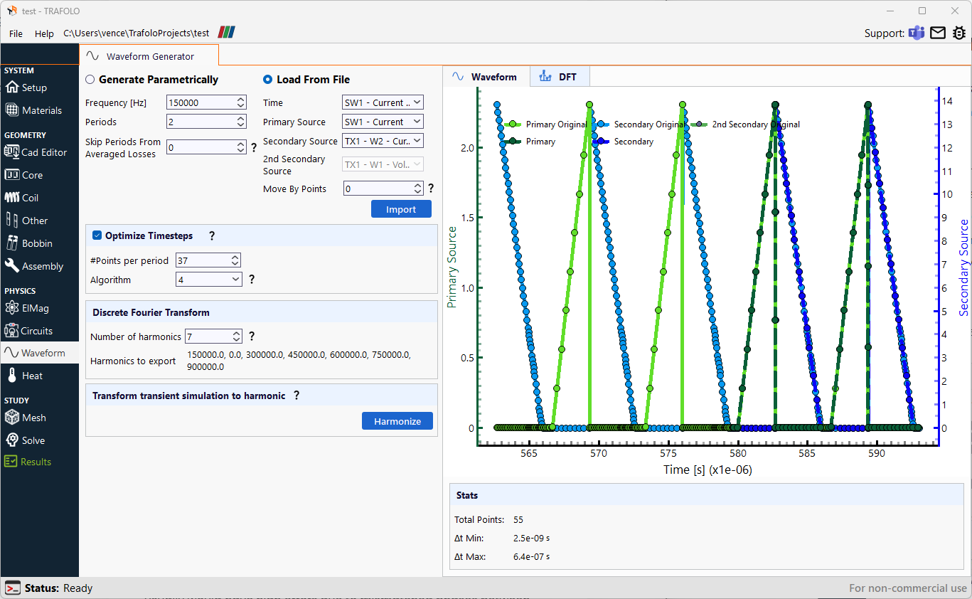
Move By Points – This setting adjusts the starting point of the waveform. To minimize mismatched phases between magnetic flux in the core and current/voltage that leads to inrush currents or voltage spikes, we can move waveforms such that the phase of current or voltage corresponds to the phase when the magnetic flux is 0. Read more in our article about inrush currents and voltages.
Optimize Timesteps
Circuit simulators often use extremely small timesteps, which can be impractical for FEM simulations. To address this, optimization algorithms redistribute the timesteps and interpolate the waveform values accordingly, ensuring more efficient simulations without compromising accuracy.
#Points per period – Number of points after waveform optimization. This is a suggested value; the actual number depends on the waveform and selected algorithm.
Algorithm – Uniform distribution (1st method) vs. gradient-based methods. The 4th algorithm is typically the most efficient, balancing steep changes in both primary and secondary waveforms. The optimized waveform should capture steep transitions while using larger timesteps where variations are minimal.
Discrete Fourier Transform (DFT)
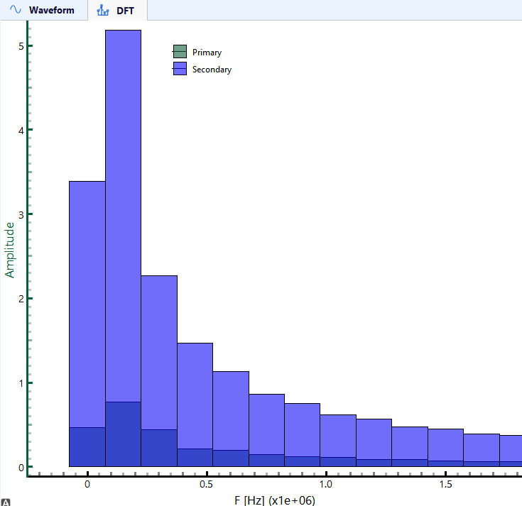
This window is available in both Harmonic simulations (via the Transient Waveform DFT window) and Transient simulations. It allows transient waveforms to be represented as a set of harmonics.
Number of harmonics
- For transient simulations, the number of selected harmonics represents those with the highest amplitudes, calculated using DFT (Discrete Fourier Transform). These harmonics are used to compute the effective Rac/Rdc coefficients in litz/stranded windings, with weights based on harmonic amplitudes over the entire period. These coefficients can be reviewed in the “Proximity Coefficients” section of the Results->Summary tab. Refer to Results for more info.
- If the user converts a transient simulation into a harmonic one by using the “Harmonize” feature, this number will indicate how many harmonics are transferred for the harmonic simulation. The software automatically adjusts the simulation type, setting the appropriate frequencies, excitations, and phases.
Transform transient simulation to harmonic – Transform a transient simulation into a harmonic one using harmonics derived from the DFT step. This option adjusts the simulation settings, switching to harmonic mode, which is advantageous when seeking steady-state solutions without inrush effects or when solving waveforms that a few distinct harmonics can represent. This can simplify the simulation process, focusing on periodic behavior over complex, time-dependent dynamics.
Effective secondary waveforms – This option is available only when the 2nd secondary winding is enabled. Typically, two secondary windings are connected to diodes in series, allowing current to pass in one direction. To obtain the correct amount of magnetizing current for each frequency used in core loss calculation, TRAFOLO computes an effective waveform for both secondary windings.
Further Reading
For deeper insights into transient modeling, please refer to the Transient Waveforms User Guide.